top of page
SVD or USV pledges to be a better form of grasping the scalar properties of the [matrixial] polynomial system, because it works directly with the once covered spectral components of it. On request, at any time SVD can return the original matrixial elements back in original positions and magnitudes, by linear algebra reconstructions, as theoretically defined as the Canonical form of the very first delivered matrix.
Here, the S and V matrices matters most.

Beta μ

The S Matrix, a Diagonal Matrix, exhibit a set of eigenvalues in decrescent order of magnitude. This must be emphasized, as the further automatic calibration process make use of such property to truncate the parameter selection to a certain measure of most influential elements of concern.

The V Matrix, a Modal Matrix, holds a set of eigenvectors, representing the current system polynomial solution.
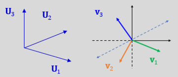
The U Matrix got the components of another orthogonality for this system.
Both this matrixes rotates the axis for the transformed scalar vectors, while the diagonal S matrix just stretches it.
The V matrix first two columns embrace the solution space, while any amount of remaining vectors come in association (add together), as a representation of what is called “the null space n dimensional vector”, for the remaining, intelligible, 3-th Cartesian coordinate system.
A real problem reaches, easily, [ 300 x 300 = ] 10^5 matrixial elements. In this context, the dimensionality between the two complementary matrixes (W1, W2) of the modal V matrix divided columns (vectors) varies dynamically, each sectioned part representing, as a heaped conjunction of new vectors, the solution and null space, respectively.
bottom of page