top of page
Here comes again our well-known modelling equation:
We got the observation Heads
and parameters (vectors) sandwiching
the model covariance matrix


Then see the
model per se,
... those
components comes as the
U, S, V vectors.
Try to produce a kind of dynamic form a thinking, which the beacons used to define the concepts not being strogholds for the need to remember it.
Being not fixed the relationship within the inner elements of this design matrix,
...
imagine how the components (USV) of the Z matrix need to act to conform, to buffer, the invisible ties connecting
a set of observations
to a set of parameters.
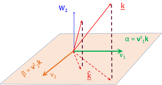
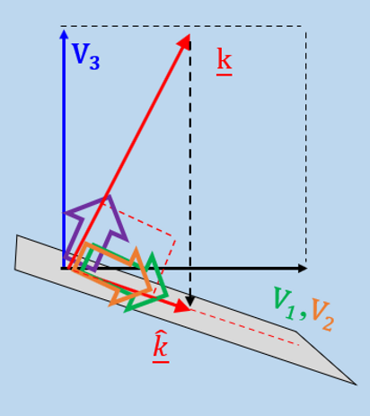
The Z matrix arrives graphically, in 3D form, as the vectors W1[v1, v2] spanning the parameter space,
while a remaining "combination"
of associated vectors - W2 [v3] spans the solution (null) space.
Examine a certain naive interpretation of it.

The X matrix SVD decomposition process starts delivering a set of eigenvalues as multiple or scalar components for the diagonal of the S matrix [λ] .
These singular values are then used to derive complementary solutions for the polynomial system at stake (the V matrix elements in parameter space).
Then another linear algebra arrangement takes care in finding the U matrix elements, as unitary vectors for the null space V matrix .
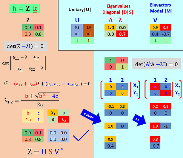
Beta μ
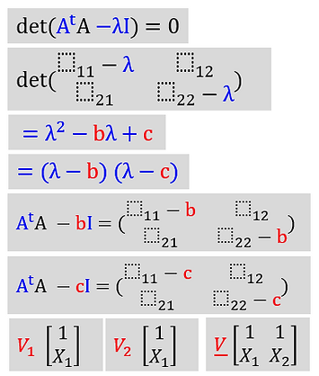
The determinant of the simplest 2 x 2 example in question (Z1[4,8]; Z2[8,4]) provides the scalar singular values (λ1,2) that, subtracted from the original of Z matrix places itself as the B representant of BX=0 relation which, in its turn, gives matrix V eigenvectors (X1, X2) through simple rules of row reduction. Finally, another interlaced orthonormal U matrix, places the unitary vectors in the null space.
The mathematical expedient of these SVD transformations were thoroughly presented here. Other option for bigger polynomials is provided as well, by MS Excel Add-in matrix.xla (page 08)


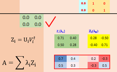
Below, the spectral components of SVD analysis are used to the back reconstruction of original Z matrix.
Finally, after the decomposition of the present 2x2 example, a expedite analysis took the licence to compare, as physical distances on the cardinal system, the different shapes formed by plotting the original vectors (columns of matrix A) end related eigenvalues (λ), after the cadential multiplication of the original matrix by itself.
bottom of page