top of page
From numerical well-posedness of the problem, to [Tikhonov and SVD] methods of regularization, we plan to pass through referential beacons as the Covariant Matrix of Parameter Error, the Covariant Matrix of Prediction Error, and so on, till the definition of the Uniqueness of a Solution by the Minimum Error Variance.
Following the trumpeted sequence, from time and again the number of estimable parameters has always been handicapped by the number of data observations. I.e. The well-posedness of all numerical problems relied in the need of a square matrix that would allows its inversion.
Once inverted we got the estimeted parameters (^ p), from heads (h)
Manual regularizations was then required in the need to a reazonable numerical scenario, from which after some algebric manuvers arrives the difference between real and estimable parameters.
It must be also said that besides [ε] there is another hidden error [e], add by the assumed numerical simplifications of this first scenario.

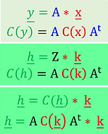
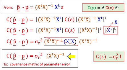
Following the propagation of uncertainties rule, where you do not need to know the contents (xi) of vector (x), to derive the intern degree of statistical correlation of an associated vector (y), comes The Covariance Matrix of Parameter Error, a spatialized conception of the uncertainties that comes in association with each estimated parameter, without knowing a priori, the noise content (ε) of a dataset.
Beta μ
P.S. For sake of simplification, this first example assume that the noise C(ε) associated with each one and between the measurements are statistically independent and that it have a even standard deviation of:
bottom of page