The Covariance Matrix of Predicted Error extends the implications of the renowned covariance matrix of parameter error in both scenarios, provided that the inversion was achievable for manual regularizations [h=Xp], a tough task to be pursued in its own.

Beyond the guarantee of having a well posed inversion problem, a further SVD mathematical regularization advantage is the conferred emphasis of having a explicit structural error term in its formulation.

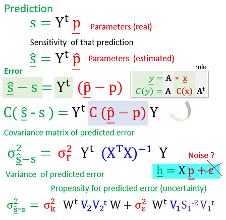
The lack a better suited approach to deal with structural error in manual (h=Xp) formulations are defended here as a problem well surpassed by the two error terms of SVD mathematical regularization, one to represent measurement noise (σ2ε), other (σ2k) to represent all the assumptions adopted to simplify the real world (countour conditions and initial parameters), in the process of handling the numerical problem.

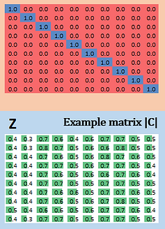
Then, take a quick look on 03 tinny modelled SVD outputs. The computed | A | B | C | determinants in the first graphic (of "volumes", actually) give us just a glimpse of how much the original Z matrix 10 vectors "scatters" the hyperspace in a decreasing scale of qualitive numerical scenarios design (see page 07).

The next graphic points out the "charge" of each singular value, the "distributed load" of structural information.

Beta μ

We know, page 08 is in badly need of an revision of applied vector analysis.

Download

SVD leads to the option of choosing how much noise will be taken in a given realization. This truncation of any response to a excellent number of singular values prevents overfitting.

This spot defines the dimensionality of solution and null spaces, the threshold of increasing potential for error in a prediction.

But some simplification assumptions (as C(k)= σ2kI) still prevents a minimum error variance solution. The Tikhonov Regularization comes to deal with this threat.

A summary of what was derived at page 13 and at page 17 shows the inverse problem's for manual and SVD mathematical aided regularizations, respectively.