Model Objectives
Up to this point, we have just discussed our case study's conceptual modeling assumptions.
In this way we placed a "space of maneuver" to all variables subjected to calibration. Starting with the delineation of all the categorical boundary conditions requirements, and ending with the fragmentation of inner constituents of the first task.
Nammelly, we got the dichotomy between model structure and parameterization.
Yes, we are looking for a collection of parameters to satisfy the model's needs in terms of its capacity to reflect the "field" expectations.
Keeping in mind that this is a interdependent processes, we also cannot ignore that, not unusually, our efforts is subjected to many failures in coming up with a meaningful solution, a situation which may indicates the lack of some crucial requirement for the system's correct operation.
Given the abundance of feasible combinations, one could argue that it is wiser to trust the calibration process to a repeatable, sufficiently supported routine to identify the optimal combinations of variables, or at least, to speed up the parameter selection process.
The more efficient the search for alternative scenarios, the better, as different conceptual models, and why not, multiple responses, can be compared for the same case.
This is the focus of the present document: - Outline, in practice, a parameterization strategy that leads to rapid calibration of numerical groundwater flow models.
Thus, let's review a few essential elements of a technique which, for instance, follows the original PEST omens “to promote the flow [... of information] between parameters and observations" (John Doherty). By the way: "the medium (the way of results achievement) is the message!" (Marshall McLuhan).
How automatic choices would be made by a software to find the best set of parameters?
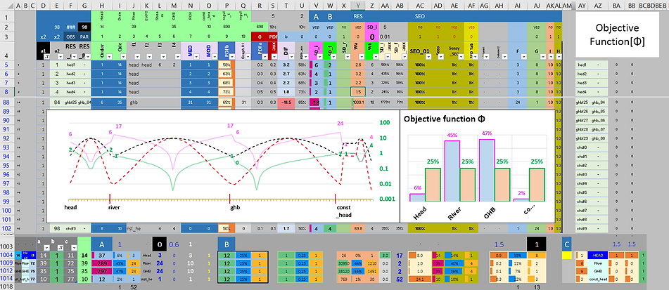
Through the implementation of instruments to guide the calibration; Via Objective Function.
Here our “virtual maquete” needs to meet the demands of 35+39+10+14 = 98 observations. And proposes to do so through a set of 35+39+10+75 = 159 parameters.
Being the model's adherence to the reality increased by bigger amounts of observations. While the greater the parameters list, the better for the algorithm to performs its choices.
Next, let's take a look at Hydraulic Heads 1 to 14 (un). That's right, measured in "units" (un). And let then be in this same measures other two linear distributions: 1 to 35 (un) of GHB and 1 to 10 (un) of CHD [Flows].
Mathematical Regularization BETAMI | PEST, theoretical foundations
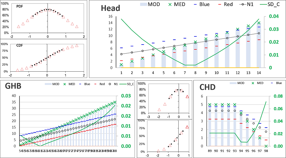
Here we go. This is the classic Gaussian functions (the bell curves) delineated from original distributions of the ... contrasts between the previously "modeled" values (MOD) and the suggestions of new one's, the "observations" (Target_N1) to be indicated by the application user regarding what is to be expected in the next model realization.
But what for?
To unequivocally comprehension of the STD curve construction process, related to the classical descriptive statistics of mean (μ), variance (σ²) and standard deviation (σ). Cause, ultimately, the point here is to determine the individual weights (W) of the so-called objective function (Φ).
Allow me to provide some guidance: The reader here is advised to take this analogy as a way to check how the extremes of the [W] curves, in green, becomes the highest weights indexes to the PEST mechanism employed in automatic selection of the best distributions of all necessary parameters, capable of, or at least attempting to, neutralize the aforementioned discrepancies.
PEST runs the model several times.
Actually, it runs one independent version of the model for each of its parameters, in a manner that permits the sensitivity vector to be extracted.
Consequently, these constituents assume the duty of specifying the magnitudes that ought to be employed in fresh endeavours MODFLOW | PEST, in order to establish the most suitable data input distributions.
Unfortunately, a single objective function (Φ) is generated by disparate groupings of information with various distributions, orders of magnitude, and measurement units.
Therefore, a correlated list of factors (commonly seen as inversely proportional to the standard deviation of the various data distributions involved), were requested in order to balance the PEST search engine.
So much so, these idealizations are seeing here as the difference between the original and balanced curves, in pink and green colors, respectively
