top of page

Let's us advance in some more concepts:
From the 3-dimentinal vector:
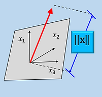
Comes its norm or magnitude
||X|| , as well,
concepts of
unity (1) and
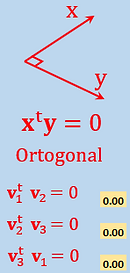
orthogonality
Meanwhile, the "covariance" model (Z) between the effective observations (h) and parameters (k) can also be described by the SVD notation:

Beta μ
It can be done because any square matrix can be seen also in terms of its canonical form, the matrixes: modal; “diagonal”; and transpose modal.
Recall the concepts of eigenvalues and eigenvectors presented in page 09.
Nevertheless, MS Excel add-ins reach the same results in:
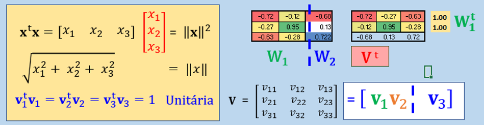
So much so, we here expeditiously introduce the implications the Partitioning of Orthonormal Matrix
Where every column is orthogonal to every other column and every column is a unit vector.

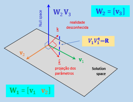
A [transpose V matrix partition] for instance, entails a 2D [solution subspace] spanned by the V1 and V2 vectors.
A little more complicated, there is also a 1D [Null subspace] spanned by V3 (or W2) vector.
bottom of page